Impulse response

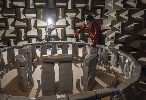
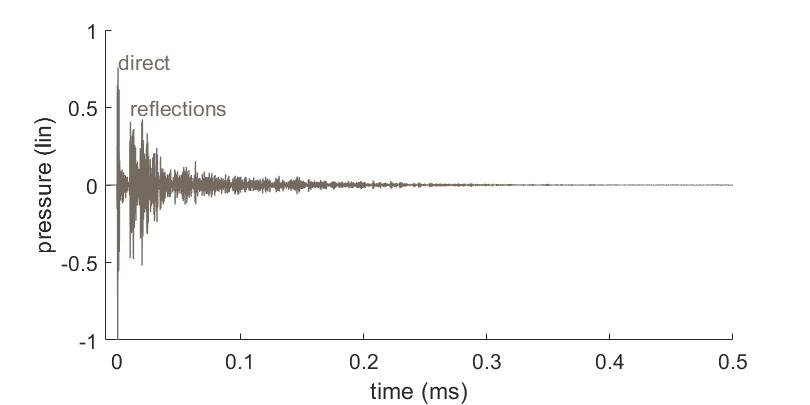
To characterise an architectural space, we measure a set of impulse response. You could measure one of these by creating a short impulsive sound and picking up the sound elsewhere on a microphone. Fig. 2 is an example from the model scale measurement for the source near the altar stone and the microphone inside the outer sarsen stones. First the sound direct from source to receiver arrives, followed quickly by a series of reflections from various stones.

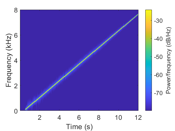
Impulsive sounds can be used, for example you can make quick room measurements by bursting a balloon. But more accurate results are obtained using a signal that sweeps through all the frequencies from low to high in a quick chirp (Fig. 3). A bit of mathematical processing then gives the impulse response.

Ultrasound

For this 1:12 scale model, we shrunk all the dimensions of the structure by a factor of 12. This means testing in the model using sound at twelve times the frequency. The reason you increase the frequency is to make the relative size of the sound waves and stone dimensions the same in the model as it would be in the real full-scale stone circle. This is vital so the sound interacts with the model stones in a way that mimics the real site at full-scale.

The chirp signal went up to 96,000 Hz, which means in theory we might get data up to about 96,000/12 = 8,000 Hz full-scale. In reality, the sources and microphones limited that range further.

Switching from the model scale measurements to the full-scale results is easy. The measurements were taken with a sampling frequency of 192,000 Hz. When we analysed we just reduced the sampling frequency by a factor of 12 i.e. 192,000/12 = 16,000 Hz.

Note, all the graphs in this blog have the times and frequencies at the full-scale equivalents.

Microphones

The 1/4″ measurement microphone we used can measure up to 100,000 Hz. The problem is that 1/4″ microphones and pre-amplifiers are noisy due to thermal and electrical noise. Broadband ultrasonic microphones with high sensitivity are not common.

This was particularly a problem for Stonehenge because it’s not an enclosed space. Consequently, a lot of the sound energy put into the model gets rapidly lost and absorbed by the walls of the semi-anechoic chamber. The way we solved this was to make measurements using 128 chirps and averaging the results to reduce the electrical and thermal noise.

Loudspeakers

Loudspeakers also pose a problem, because we require them to work over at least six octaves and be small enough to fit into the model. As we’re working beyond the audible frequency range, there are limited choices because not many people make loudspeakers that span the range we need. Bowers and Wilkins kindly gave us a diamond tweeter that we used to give the broadest bandwidth for auralisation. We’ve assumed that this has a directivity similar to a human talker, but we need to measure to check that.

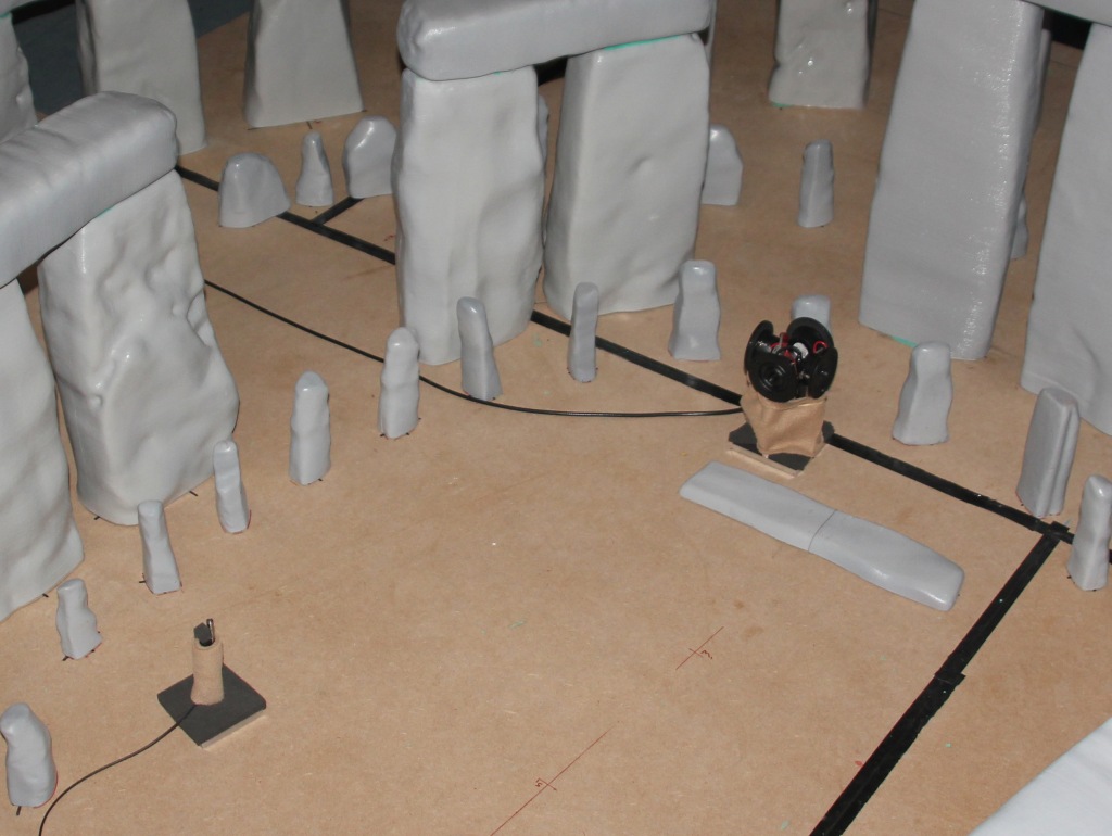
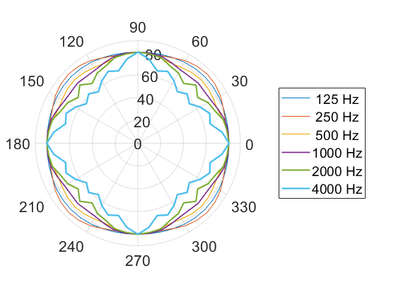
Architectural acoustics is normally tested with loudspeakers that radiate evenly in all directions (‘omnidirectional’). Consequently we arranged four ring tweeters to achieve a more uniform radiation of sound horizontally (see Fig. 5 for the directivity). The source is shown in Fig. 4 near to the altar stone.

We also used a 3.5″ tweeter in a cabinet for low frequency measurement.

Analysis

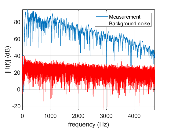
Fig. 6 shows the spectrum for the measurement vs the background noise (a measurement with the loudspeaker turned off). It shows the measurements most vulnerable to noise are at high frequency, because the impulse response naturally has less energy at high frequency. So below I just show the plots in the 4000 Hz band.

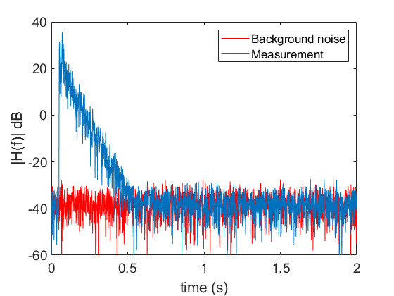
Architectural acoustic involves analysing the sound reflections as they die away. Fig 7. shows an example of this for the 4000 Hz octave band. Typically we’d want the measurement to start at least 45 dB above the background noise floor, and this is achieved in this case.

Air absorption

A key issue in scale model testing is to scale the acoustic properties. For example the stones should absorb the same amount of energy at 12,000 Hz in the model, as they would do at 1,000 Hz in the real stone circle.

An important source of sound absorption in models is air absorption. This is the loss of sound energy as the sound waves go through the air. This absorption is mostly not important in architectural acoustics, but it’s important in scale models because air absorption rapidly increases with frequency. For example the air absorption at 48,000 Hz in the model is 4 times greater than it would be at full scale 4,000 Hz.

To correct the impulse responses for air absorption in each octave band a correction curve was applied [4]. This only makes a significant different in reverberation times at 2000 and 4000 Hz, increasing the decay times by about 0.1 and 0.2 seconds respectively for the measurement example shown in this blog.

Calculating reverberation time

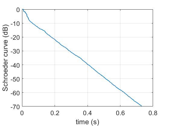
To extract the reverberation time, we first need to calculate the Schroeder curve [2]. Reverberation time is defined as the time it takes a steady-state sound to decay by 60dB once the source is turned off (the interrupted noise method). Our measurements use short impulsive sound, which is a bit different. The Schroeder curve converts the impulse measurements to the decay curve you’d get from interrupting steady-state noise.

An example is shown in Fig. 8 (details of this calculation are in the Appendix). The reverberation time is calculated by fitting a regression line from -5 to -35 dB on the Schroeder Curve [3]. In this case, the reverberation time is 0.65 s (the time for sound to decay by 60 dB).

Any measurement details I’ve missed you’d like to know? Please comment below.

What did the measurements show?

The results have now been published in Using scale modelling to assess the prehistoric acoustics of stonehenge, Journal of Archaeological Science (open access)

Appendix: More details

You only need to read this if you’re thinking of carrying out similar measurements. This is far too detailed for a casual read!

Equipment

• Laptop running Audacity for playing source signal and simultaneous record. Recording both the microphone signal and loop-back (a direct feed of the source signal from the sound card back into another channel). Loop-back used to calibrate for delays through sound-card.
• RME Fireface UFX interface running at 192 kHz sampling frequency. Note, while many soundcards use 192 kHz, many of them won’t allow you access to the audio file at this rate.
  • L9 from mic, L10 from loudspeaker input, gain set to maximise SNR. Set Instr. In Totalmix
• Home made ‘Dial-a-watt’ amplifier.
• Loudspeakers:
  • B&W Diamond Tweeter.
  • 4x Peerless XT25SC90-04 Ring Radiator Tweeter arranged in a square. Two pairs connected in parallel, then these connected in series to give a nominal 4 ohms. Middle of tweeter 1.56 m from floor.
  • 1x Dayton Audio nd91-4 3.5″ Aluminum cone full range driver in a 0.166l.
• GRAS 40BF 1/4″ Ext. Polarized Free-field Microphone.
• GRAS 26AA 1/4″ Preamplifier.
• GRAS XXX 2-Channel Power Module 336 in semi-anechoic chamber. Settings: 40 dB gain, F, high pass
• B&K 2610 Measuring amp outside semi-anechoic chamber Settings: Direct input, front B&K output, 20 dB gain

Signals and analysis:

• Logarithmic sweep generated using Angelo Farina’s Aurora Audacity plug-ins [1]
• Setting in Aurora: fs = 192kHz, 800 Hz to 96,000 Hz, amplitude 0.25 in Aurora GUI, 1s sweep, 1s silence, 128 repeats, 0.01 fade in, 0 fade out.
• The inverse sweep was created in the Aurora plug-ins, but the decorrelation processing was done in MATLAB.
• Voltages:
  • B&W tweeter: 4V peak-peak
  • 4-ring-tweeters: 6V pk-pk
  • Low frequency source: 2V pk-pk
• By analysing in octave bands we achieve the necessary signal to noise ratio (Fig. 7).
• Method for extending impulse response in each octave band to remove truncation errors from Schroeder curve:
  1. The time where the measurement meets the background noise was identified by eye (about 0.5s in Fig 7.). Call this T_N.
  2. The time at which the direct sound arrived was identified by eye. Call this T_D (about 0.08s in Fig 7.)
  3. The decay rate was estimated by a linear regression between point T_D and T_N.
  4. The measured impulse response was truncated at T_N.
  5. Gaussian noise was added from T_N to continue the decay with the same rate as the earlier decay from T_D to T_N. The standard deviation of the added Gaussian noise was set to match that in the early part of the decay (calculated with the linear decay removed).
  6. The Schroeder curve was calculated [2].
  7. The point where the Schroeder curve is 10 dB above the level at point T_N was identified (to give 10dB headroom above background noise). Steps 3-6 were repeated using this new truncation point.

Room:

• Lights off in semi-anechoic chamber to reduce high-frequency

References

[1] Farina, A., 2000, February. Simultaneous measurement of impulse response and distortion with a swept-sine technique. In Audio Engineering Society Convention 108. Audio Engineering Society.

[2] Schroeder, M.R., 1965. New method of measuring reverberation time. The Journal of the Acoustical Society of America, 37(6), pp.1187-1188.

[3] ISO 3382-1:2009. Acoustics. Measurement Of Room Acoustic Parameters. Performance Spaces.

[4] Ismail, M.R. and Oldham, D.J., 2005. A scale model investigation of sound reflection from building façades. Applied Acoustics, 66(2), pp.123-147.

[5] Trevor J.Cox, Bruno M.Fazenda and Susan E.Greaney. Using scale modelling to assess the prehistoric acoustics of stonehenge. Journal of Archaeological Science. Volume 122, October 2020, 105218. https://doi.org/10.1016/j.jas.2020.105218

Follow me

• 
• 
• 
•